NeurIPS 2026 Spotlight

The Neural Race Model

Stimulus-conditional stochastic accumulation, trained end-to-end on how people choose and how long they take.

Omar Ghezzi1Alessandro D'Amelio1Vittorio Cuculo2Rita Cucchiara2Giuseppe Boccignone1
1University of Milan2University of Modena and Reggio Emilia
omar.ghezzi@unimi.italessandro.damelio@unimi.itvittorio.cuculo@unimore.itrita.cucchiara@unimore.itgiuseppe.boccignone@unimi.it
Stimulus
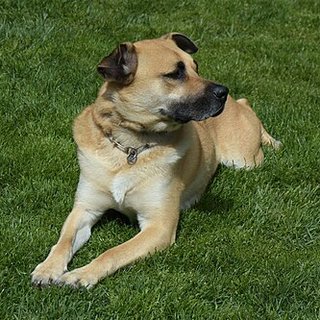
Stimulus shown on this trial
dog clarity –
Evidence for four alternatives accumulates until one hits the bound.

Each trial draws a new stimulus (the image beside the race). It sets the drift of every accumulator and the height of the bound: a clear image drives its own accumulator hard and the race ends early, a degraded one (blurred, noisy) leaves the evidence weak and ambiguous, so the race runs longer and errors become more likely.

Why this matters

A perceptual decision takes time, and that time is data. For fifty years, race and drift-diffusion models have explained choices and reaction times with a few interpretable parameters, but they are blind to the stimulus itself: whatever an image contains must first be squeezed into a single number such as "coherence".

Deep networks, on the other hand, see images but not time. Existing image-computable reaction-time models read out a proxy (confidence, entropy, the number of recurrent steps or FLOPs) that correlates with RT and must be rescaled to milliseconds afterwards.

The Neural Race Model keeps the race. It is a neural stochastic differential equation in which one accumulator per alternative races in continuous time towards a learnable, stimulus-dependent threshold. Drift, diffusion and threshold are neural networks conditioned on a stimulus embedding, and the whole model is trained end-to-end on the joint likelihood of human choices and reaction times.
0.834vs 0.840 human

Scene categorisation accuracy, within 0.006 of the human noise ceiling and the closest of all models.

0.989vs 0.971 human

Chronometric correlation on random-dot motion: the model's RT curve across coherence matches human median RTs.

3 of 3conditions

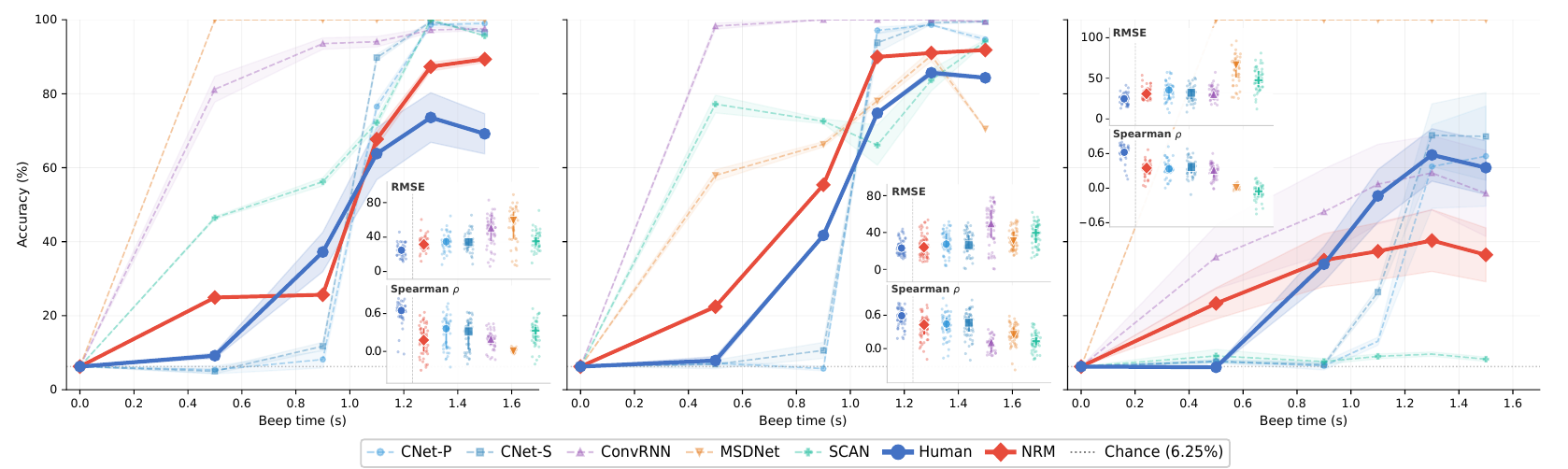
Lowest speed–accuracy curve error on SATBench, with a single model and no per-deadline refitting.

msnot a proxy

Reaction times come directly from a first-passage event, in physical time, with no post-hoc rescaling.

How it works

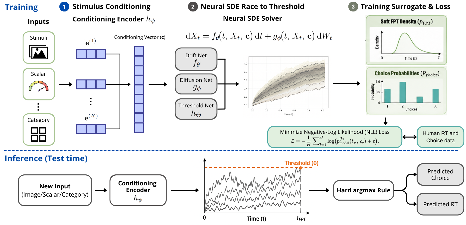
The evidence state Xt ∈ ℝN holds one accumulator per alternative. A conditioning encoder turns the stimulus into a vector c, which parametrises every part of the race:

dXt = fΞ(t, Xt, c) dt + gφ(t, Xt, c) dWt,    Θ(c) = exp hΘ(c)

NRM pipeline. Top: training, where inputs are encoded into a conditioning vector that parametrises drift, diffusion and threshold networks of a neural SDE, with a soft first-passage surrogate and an NLL loss against human RT and choice data. Bottom: inference, where a hard argmax over first crossings yields predicted choice and RT.
Training (top) uses a smooth first-passage surrogate so gradients flow through the stochastic race. At test time (bottom) the surrogate is removed and the classical hard race produces the choice and the reaction time.
  1. Condition on the stimulus

    A modular encoder maps images, videos, scalars or categories to c. For video, ct changes at every integration step.

  2. Race in continuous time

    Neural drift and diffusion push the accumulators; a neural threshold sets the bound, so urgency can depend on what is seen.

  3. Smooth the finish line

    A sigmoid of width 1/Îș replaces the hard crossing. Monte Carlo trajectories give a soft first-passage density and choice probabilities, trained by NLL through the stochastic adjoint.

  4. Race for real at test time

    The surrogate is dropped. The first accumulator to cross Θ gives the choice; the crossing time gives the RT.

Play with a race

Below is a two-alternative race of the kind the NRM generalises. Stimulus strength raises the drift of the correct accumulator. Watch the two signatures of human decisions appear: stronger evidence gives faster and more accurate choices, and a higher bound buys accuracy at the cost of time.

correct accumulatorincorrect accumulatorthreshold Θhistogram: correct above, errors below
Like motion coherence: how much the stimulus favours one side.
Raise it for caution, lower it for speed.
–
accuracy
–
median RT
–
median RT, correct
–
median RT, errors

In a classical model, "stimulus strength" is one hand-picked number per trial. In the NRM, drift, noise and threshold are all computed from the stimulus embedding itself, so two images with the same nominal difficulty can still produce different races.

Making the finish line differentiable

A hard threshold crossing has no useful gradient. The NRM replaces it with a soft crossing probability σ(Îș(X − Θ)), takes the positive increments of that probability along each simulated path, and averages over M trajectories to obtain a soft first-passage-time density. As Îș grows, the soft density converges to the true one, at rate O(√Δt + 1/Îș + 1/√M).

Drag Îș to see the trade-off: small Îș gives smooth gradients but a smeared, shifted density; large Îș is exact but noisier to differentiate. The paper shows the budget-optimal sharpness scales as Îș⋆ ∌ M1/3.

soft crossing band, width ~1/Îșsoft FPT density (training)hard FPT histogram (test)
The paper trains with Îș = 100.
Bin-wise noise shrinks like 1/√M.
–
distance to hard density (total variation)
–
mean RT shift, soft minus hard

Results on three benchmarks

The NRM is compared against classical sequential-sampling models (LNR, LBA, DDM), image-computable RT models (RTify, cRNN) and anytime-prediction networks (CNet, ConvRNN, MSDNet, SCAN). Human curves are shown as a noise ceiling.

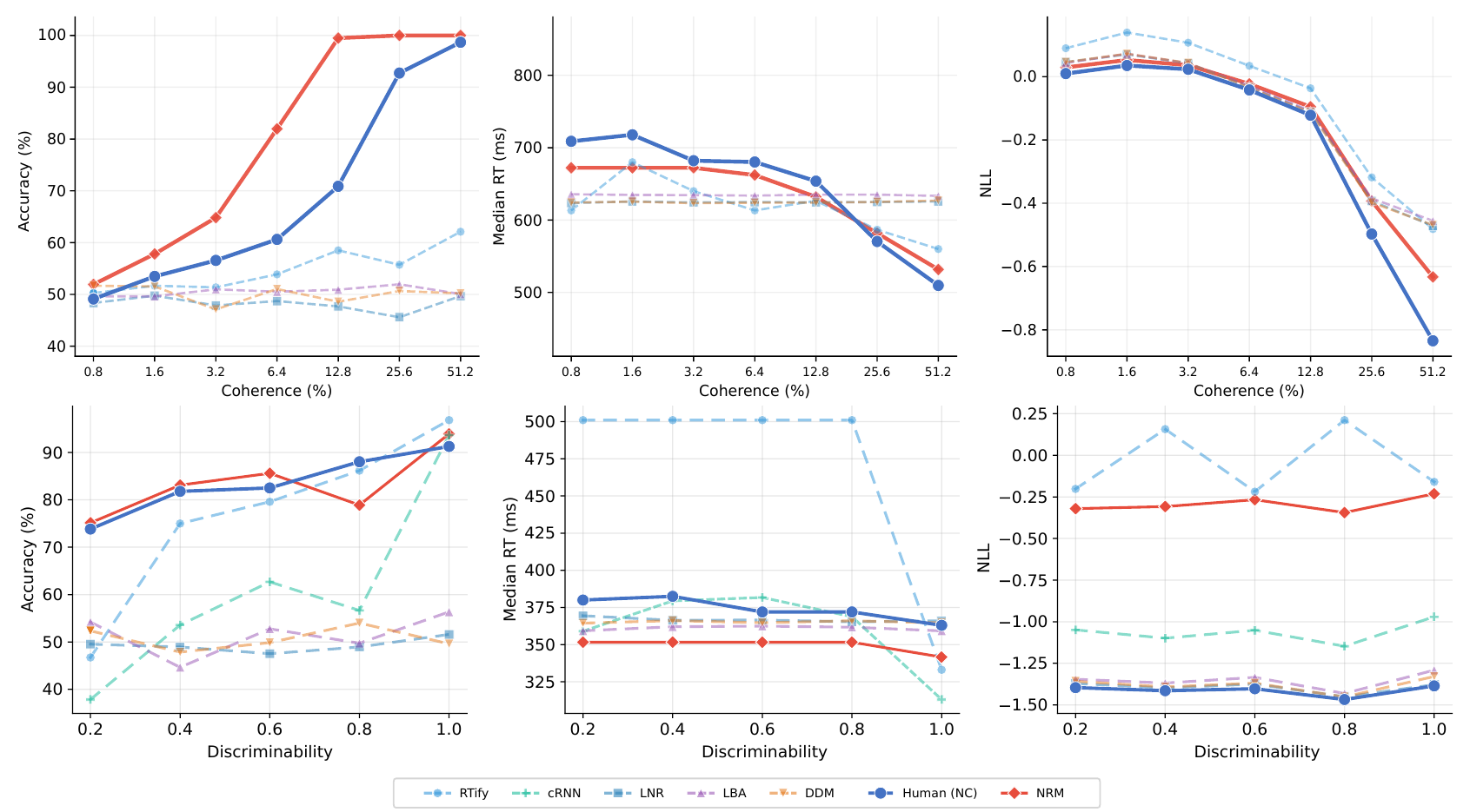
Videos of moving dots at seven coherence levels, 21 observers. The NRM is conditioned on a time-varying motion-energy signal and is the only model that reproduces both the rising psychometric curve and the falling chronometric curve.

Accuracy vs coherence

Median RT vs coherence (ms)

Global results: accuracy 0.794, Îș 0.585, best RT likelihood (NLL −0.147 vs human −0.204). The NRM overshoots human accuracy at high coherence.

Show the full figures from the paper
Figure 2 of the paper: accuracy, median RT and NLL curves for the random-dot motion task (top) and the scene categorisation task (bottom), comparing NRM with baselines and the human noise ceiling.
Random-dot motion (top) and scene categorisation (bottom): accuracy, median RT and NLL for every model against the human noise ceiling.
Figure 3 of the paper: speed–accuracy trade-off curves for Color and Blur, Color and Gray, Gray and Noise conditions, with RMSE and Spearman insets.
SATBench speed–accuracy curves for Color & Blur, Color & Gray and Gray & Noise.

Watch the trained model decide

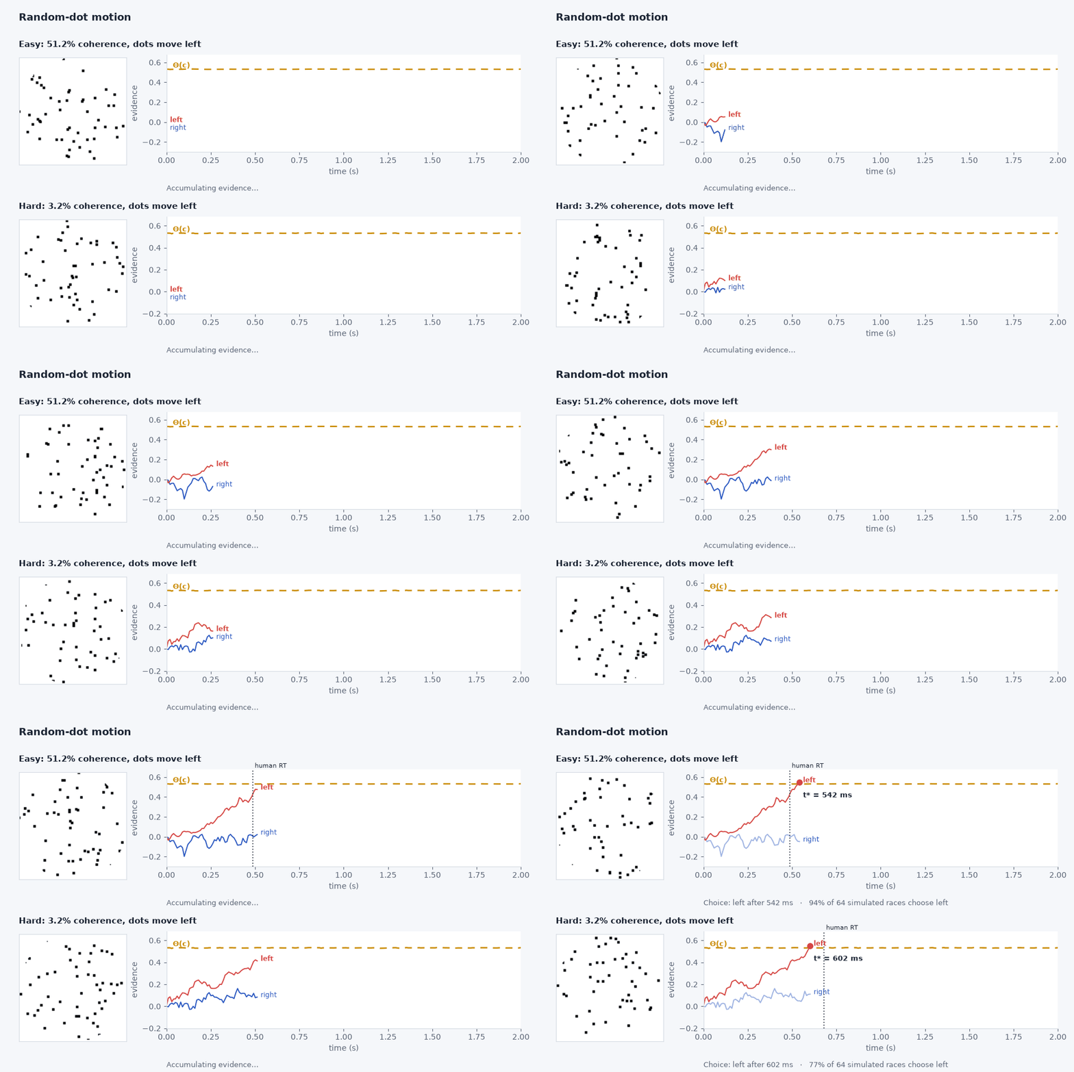
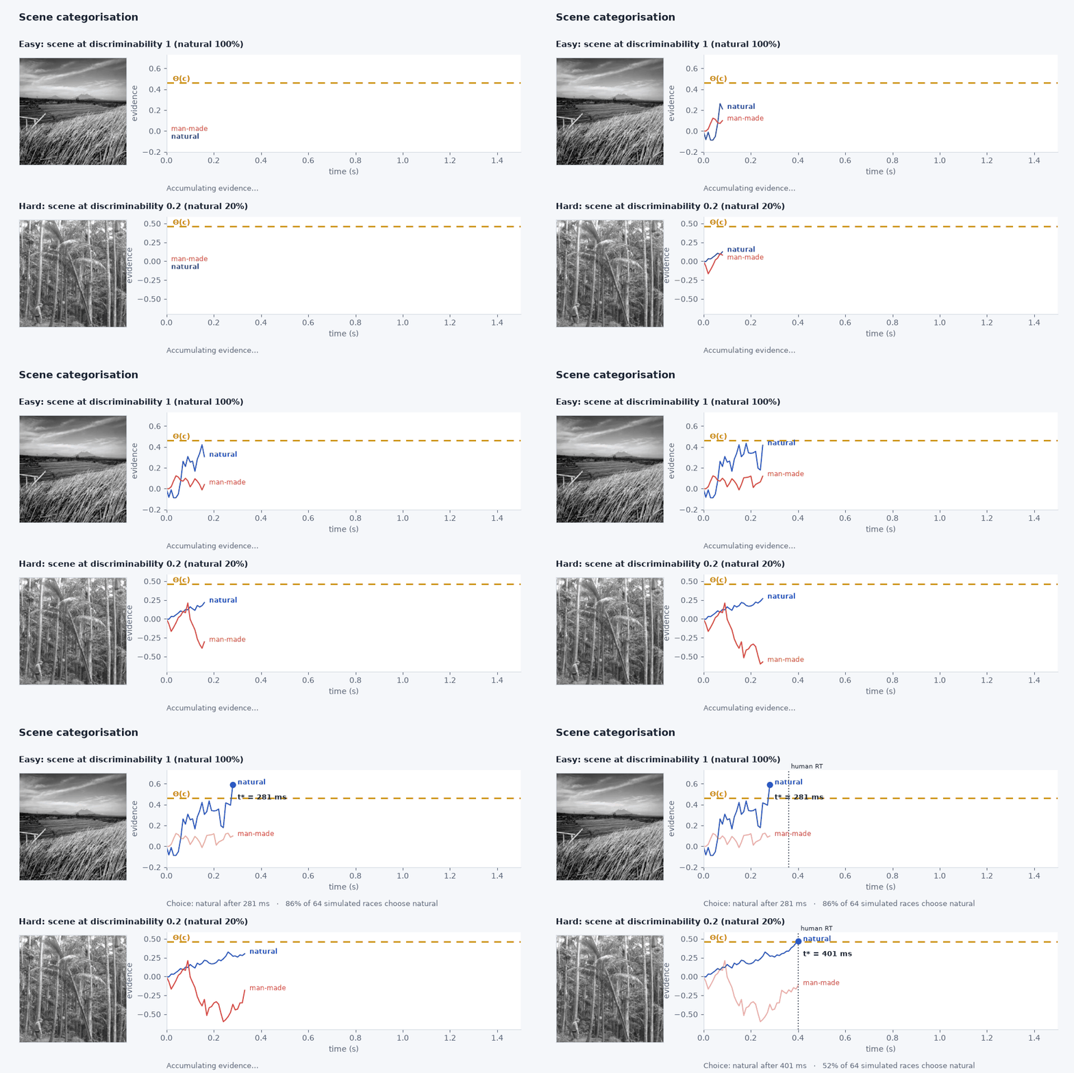
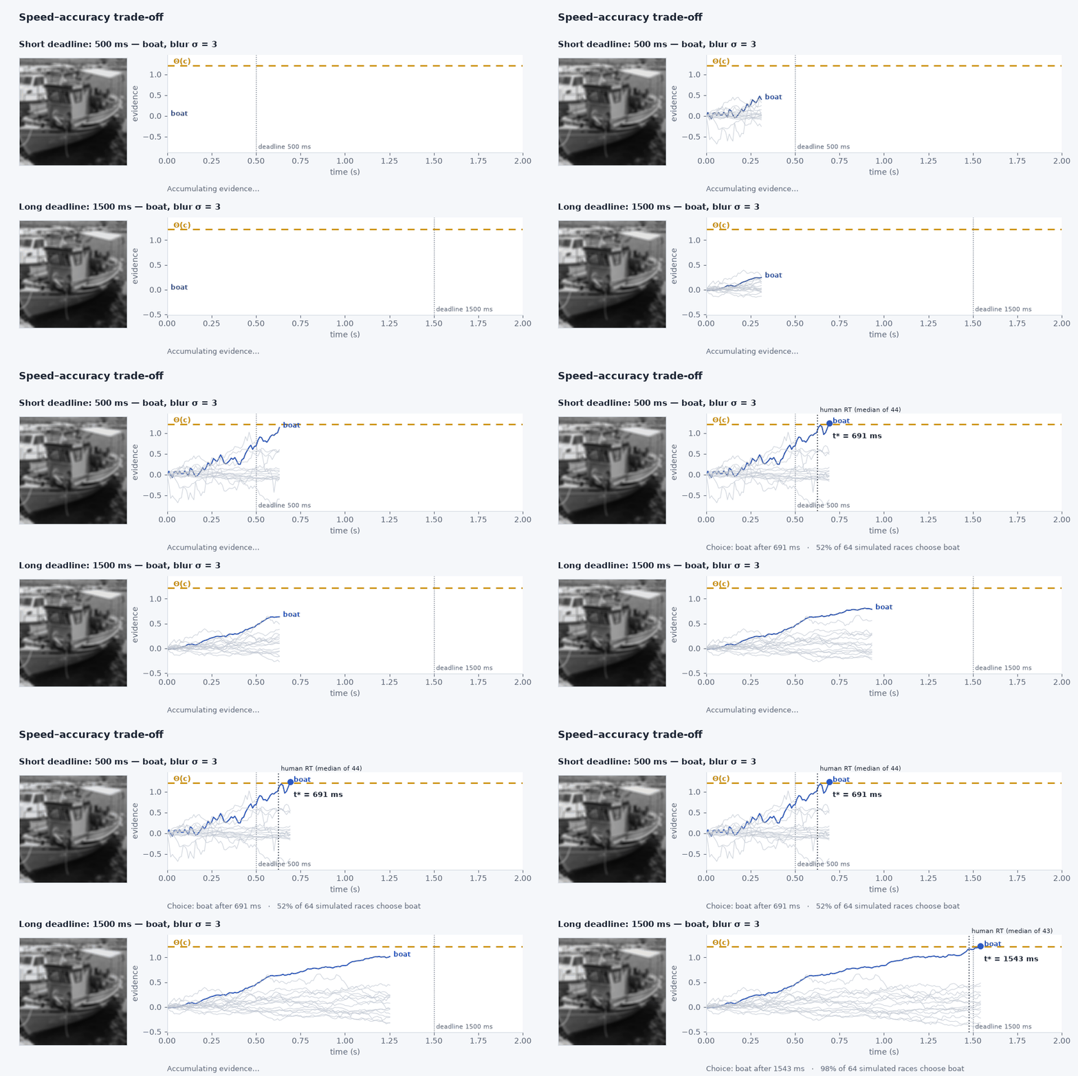
Each animation is the released NRM on two held-out test trials, one easy and one hard. Beside the stimulus runs one sampled race: the accumulators, the bound Θ(c) the model computes from that stimulus, its crossing time t* and the human RT for the same stimulus. Below each race, the share of 64 simulated races that pick the correct answer.

Dots drifting left at 51.2% and at 3.2% coherence. The motion-energy embedding changes frame by frame, and so does the push on each accumulator. With clear motion the left accumulator reaches the bound in about half a second and 94% of races choose left; at 3.2% the two stay close for longer and the share drops to 77%.

Two random-dot motion trials, 51.2% and 3.2% coherence. Beside each dot video, the race of the left and right accumulators towards the bound, with the model's crossing time and the human RT.
The dots are drawn at 60 per frame instead of the experiment's 6, for legibility; the race is the model's response to the real trial.

Readable in the language of the brain

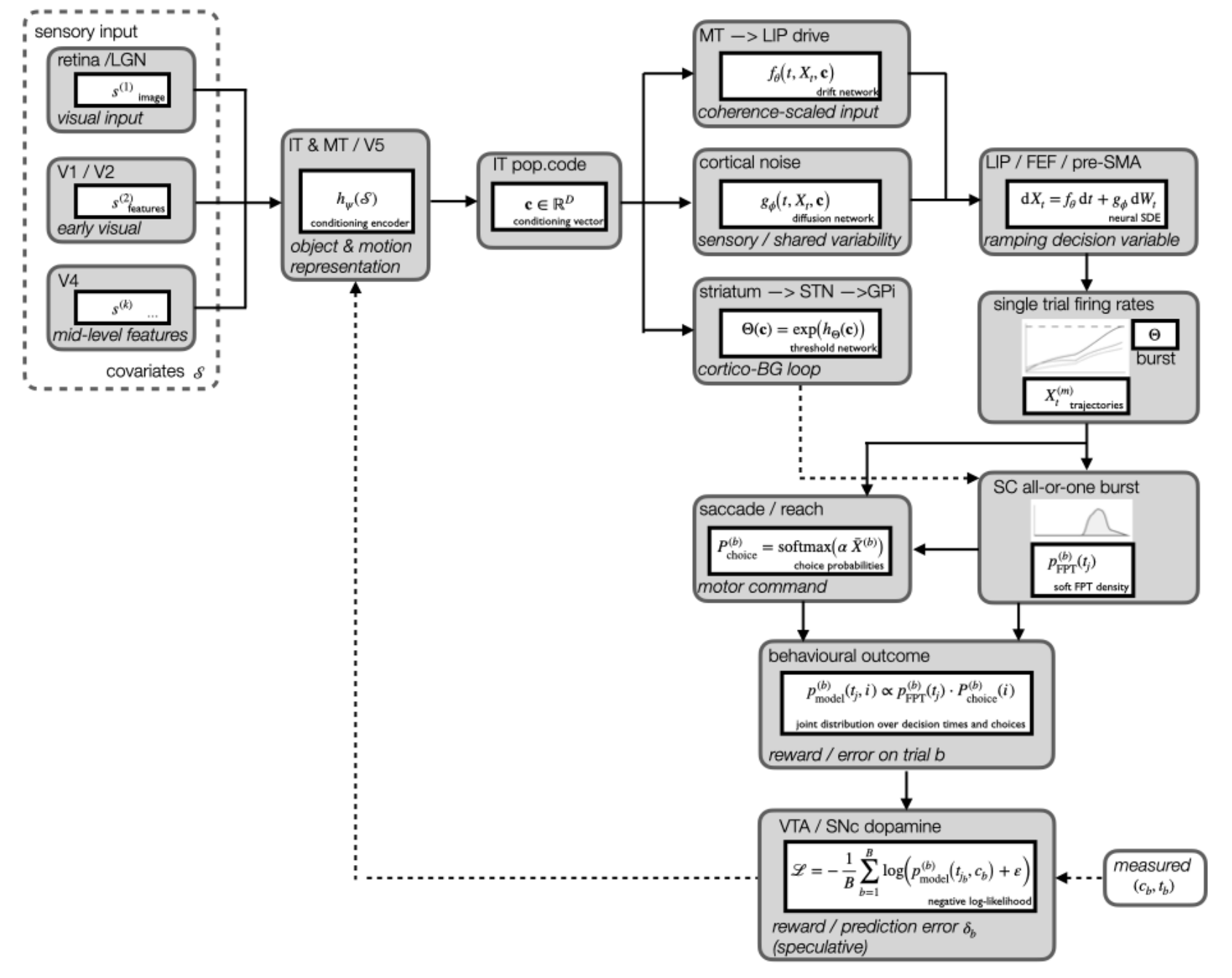
Because the NRM keeps the accumulate-to-bound structure, each component has a natural counterpart in the primate decision circuit. The paper offers this as interpretive commentary, not a mechanistic claim, and marks where the analogy breaks.

NRM componentApproximate substrateHow close
Encoder hψVentral stream V1→V4→IT; MT/V5 for motionpartial: frozen, feedforward
Drift fξCoherence-selective MT→LIP drivestrong
Evidence XtLIP, FEF, pre-SMA ramping; human CPP (EEG)strong
Diffusion gφStructured, shared cortical variabilityopen question
Threshold Θ(c)Cortico-basal ganglia loop: striatum, STN, GPistrong
First passage t*Superior colliculus all-or-none burst; FEFstrong
Show the circuit schematic
Schematic mapping NRM components onto the primate perceptual decision circuit, from sensory input through IT and MT, to LIP, the cortico-basal ganglia loop, superior colliculus and dopamine.
NRM components placed on the primate perceptual-decision circuit (Appendix D of the paper).

Cite

@inproceedings{ghezzi2026neuralrace,
  title     = {The Neural Race Model},
  author    = {Ghezzi, Omar and D'Amelio, Alessandro and Cuculo, Vittorio and
               Cucchiara, Rita and Boccignone, Giuseppe},
  booktitle = {Advances in Neural Information Processing Systems (NeurIPS)},
  year      = {2026}
}